Amazon Redshift is a fully managed peta byte scale datawarehouse designed to handle large scale datasets, perform data analysis and business intelligence reporting.Redshift delivers fast query performance by using columnar storage technology to improve I/O efficiency and parallelizing queries across multiple nodes.
The scope of this article is to share the table design practices which showed significant performance improvements.
Architecture
Amazon Redshift is based on MPP architecture in which cluster is the core component. A cluster is composed on leader and compute nodes.
**Leader Node: **Coordinates the compute nodes and handles external communication.
-
SQL endpoint to the cluster
-
Stores metadata of objects in the cluster
-
Performs aggregations and user communication
Compute Nodes: Complies the elements of execution plan, executes the code and sends the intermediate results to the leader node for completion.
**Spectrum Nodes: **Execute queries directly against Amazon Simple Storage Service(S3). Scaling of spectrum queries depends on number of slices and node type of the redshift cluster.
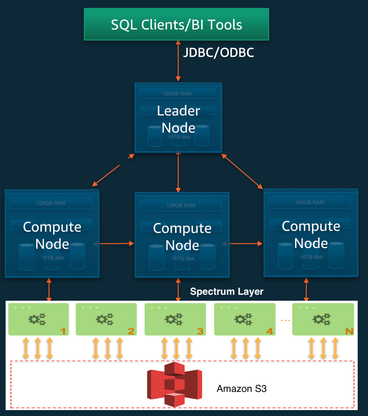 Redshift Architecture
Table Design Principles
Redshift is designed under the principles of Massively Parallel Processing (MPP) which is different from traditional datawarehouses. Indexes, Partitions, constraints (PK, FK) are often used in the traditional databases to improve query performance but redshift table natively doesn’t have indexes or partition keys.
Below are the important properties of a redshift table which will directly contribute to its query performance.
-
Data Sorting
-
Data Distribution
-
Data Compression
-
Constraints
Let’s deep dive into each of these sections.
Data Sorting
Amazon Redshift stores the data on disk in sorted order based on sort key of the table. There can be one or more of columns as sort keys for a table. But how does sorting the data in disk improves the query performance? The answer is ‘Zone Maps’.
Zone Maps: It’s an in-memory block metadata which contains information about per-block min and max values. Redshift stores columnar data in 1 MB disk blocks.
When a query uses range restricted predicate the query processer uses in the min and max values information from zone maps to rapidly skips large number of blocks during table scans which improves the query performance as amount of scanned data is reduced.
For example, Let’s take DW table with 5 years of data sorted by a date column. Queries running with the date range for a week with skip 99 percent of disks blocks from the scan.
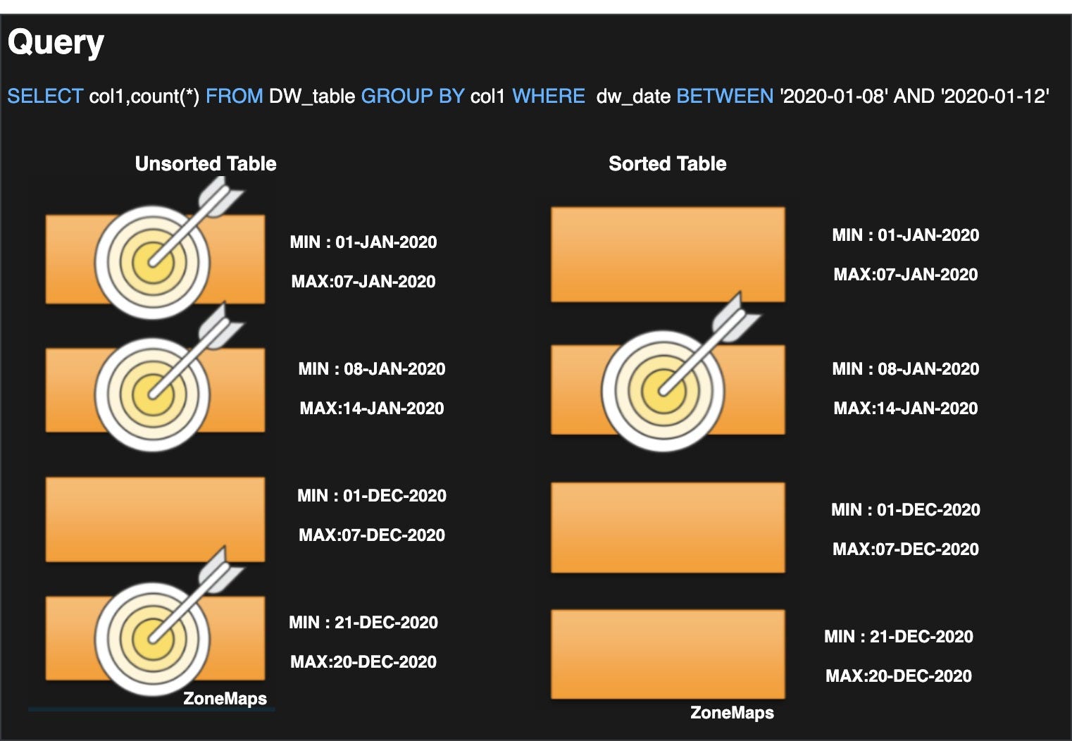 Zone Maps in Redshift
There are two types of sort keys:
Compound Sort Key: Component sort key is made up of all columns list in the sort key definition. Its most useful when a query’s filter applies conditions, such as filters and joins, that use a prefix of the sort keys. On contrary the performance of component keys decreases when queries depend only on secondary sort columns, without referencing the primary columns. Compound is the default sort key.
Interleaved Sort Key: Interleaved sort gives equal weightage to each column, or subset of columns, in the sort key and it’s based on Z-order curve concept. Its most useful when queries use restrictive predicates on secondary sort columns
Best Practices: Sort Keys
- Create sortkey based on frequently filtered columns by placing the lowest cardinality column in the first.
· On most fact tables, the first sort key column should be a temporal column
· Columns added to a sort key after a high-cardinality column are not effective
-
Check the Unsorted column % of table unsorted in SVV_TABLE_INFO. Higher number indicates the need of VACUUM.
-
Check Compression of sort key column in **skew_sortkey1 **column . Too much compression in sort key leads to increase in records scan and leads to performance impact
Design considerations:
-
Sort keys are less beneficial on small tables
-
Define four or less sort key columns — more will result in marginal gains and increased ingestion overhead
Data Distribution
Distribution style property defines how the table’s data is distributed throughout the cluster. Distributing the data spread across the compute nodes will result in high degree of parallelism, minimize data movement across nodes (same as shuffle behavior) and avoid data skewness. There are three types of distribution styles in redshift.
**Even Distribution: **Round robin style of data distribution. One row per slice is loaded.
**Key Distribution: Columns defined as DISTKEY **is used to group the records together on one slice and loaded. This method is effective when redistribution needs to be avoided. For example, if product_id is choose as distkey for sales table then all sales related the product_id is stored in the same node.
**All Distribution: **All the data in the table resides on the first slice of every node. Data is duplicated across all the nodes in the cluster. This type of distribution is suitable for small dimension tables as local joins are enabled at the compute node level.
Best Practices: Distribution Key
Selecting a key for distribution plays a vital role in the table’s access pattern. Redshift suggests to go in the below order while choosing the distkey
- Choose** DISTSTYLE KEY **is optimal for tables with use cases with
· **JOIN **performance between large tables
· **INSERT INTO SELECT **performance
· **GROUP BY **performance
The column that is distributed should have high cardinality and not cause data skewness. Below query can be used to check the value
- Choose **DISTSTYLE ALL **is optimal for tables with use cases with
· Optimize **JOIN **performance with dimension tables
· Reduces disk usage on small tables
· Small and medium size dimension tables (< 3M rows)
- Choose **DISTSTYLE EVEN **only when table use cases are unknown and above option are ruled out. It the default DIST style.
Compression Encoding
Redshift being a columnar database enables compressions at the column-level that reduces the size of the data when its stored. Compression conserves storage space and reduces the size of data that is read from storage, which reduces the amount of disk I/O and therefore improves query performance.
Compression can be applying to a table two ways.
-
Manually chosen compression algorithms for each column during table creation
-
Use COPY command to analyze and apply compression
Redshift strongly recommends COPY to apply automatic compression.
[ANALYZE COMPRESSION](https://docs.aws.amazon.com/redshift/latest/dg/r_ANALYZE_COMPRESSION.html) command comes handy to for choosing the optimal compression encoding manually for custom use cases
Best Practices: Compression
-
Apply compression to all the tables
-
Avoid compressing SORT KEYS in the table
-
Changing column compression requires table rebuild. Column encoding utility available here.
Constraints
Constraints are not enforced by Redshift. Redshift assumes all keys in validated when loaded with an exception of NOT NULL column constraints
Constraints should be enforced prior to loading into the cluster.
Redshift highly recommends to define constraints as Query planner uses PK and FK in certain statistical computations.
Summary
-
Sort keys should be added on the potential columns that will be used in query filters. Column order matters.
-
Avoid compressing the sort key column to reduce data scan.
-
Avoid distribution keys on columns with low cardinality.
-
Use ANALYZE COMPRESSION to choose the optimal compression for the columns.
-
Always use table constraints for better query planning.
-
Identify sort key metrics using system tables (SVV_TABLE_INFO)
Resources
https://github.com/awslabs/amazon-redshift-utils https://docs.aws.amazon.com/redshift/latest/dg/welcome.htmlhttps://aws.amazon.com/blogs/big-data/amazon-redshift-engineerings-advanced-table-design-playbook-compound-and-interleaved-sort-keys/